Intro: Welcome to the Deep End

If you’ve delved into the first three instalments of this series, outstanding, and by doing that, you possibly now have a bit of an understanding of how a teenager, back in the day, on an Amiga, has now evolved to solve and build real-time, intelligent 4K conversion tools for broadcasters. Helping to define what “filters” can actually be and provide, and why your TV’s built-in upscaler is basically the Swiss Army knife of video processing: handy, but not exactly surgical. But now it can.

So, at this time, we thought we’d go deeper.

Think of this as a  “backstage tour.” A tour where you get to see the machinery the audience never sees: the decoders, the GPUs, the AI models, pixel blocks that dance across every frame, the tone curves that stop bright stadium lights from turning into supernovas—all generating clarity.

This article walks through the full Pixop LIVE pipeline, from decoding compressed streams into raw pixels, through restoration and super-resolution, to real-time GPU optimisation, SDR-to-HDR conversion, training strategy, and the architectural choices behind Pixop’s models, before closing with a look at diffusion models and what comes next.

And because sports is where demand is high and where Pixop LIVE is often deployed first, with ultra-compressed feeds, fast action, and complex motion, we’ll use many sports examples throughout this discussion. Also, whether you are in sports broadcasting or not, you probably already know what I’m talking about.

Here’s the question we’ve been working towards answering:

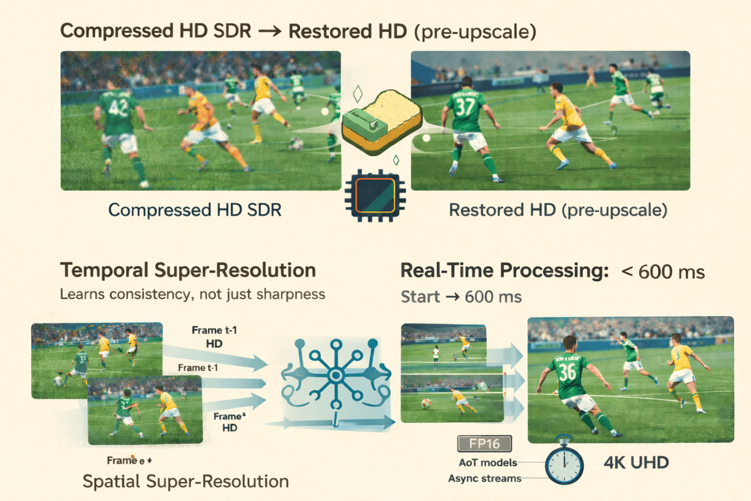
How do you transform a highly compressed HD SDR football feed into crisp 4K HDR, where the extra pixels enhance the viewer’s experience, all within under 600 milliseconds, consistently, frame after frame?

That’s what we’ll address in the rest of this article.

1. From Compressed Stream to Raw Pixels: The Starting Line

When I asked Jon to describe the pipeline from start to finish, he smiled and said:

“It’s not magic. It’s just math trained to make smart guesses.”

However, the first step is actually not smart at all. It’s brutally simple.

Step 1: Decode

Pixop LIVE sits inside a transcoder, currently an open-source one, with a very permissive licence. It receives a compressed video stream (H.264, HEVC, sometimes even MPEG-2 for legacy feeds), and the decoder turns it into raw RGB frames.

Yes, that means fully uncompressed bitmaps.

If your source was a 1080p50 football match, you now have 50 giant images every second, each one about 8MB in floating-point RGB. These are moved directly into GPU memory because everything from here happens on the GPU.

Step 2: Quantise to FP16

The frames arrive as 32-bit floats, but to run the AI fast enough, we convert them to 16-bit (FP16) internally.

Do we lose detail? A tiny amount. Jon tested it extensively:

“It’s only a few per cent difference. Surprisingly little. And the performance gain is massive.”

FP16 is the difference between real-time and “wait two seconds per frame.”

Sports broadcasters don’t do “two seconds per frame.”

Now the fun begins.

2. Stage One: Restoration, Where 90% of the Compute lives

TLDR: sports feeds can be messy and need cleaning up before even considering upscaling. In fact, almost no broadcast HD feed is consistently stable or predictable.

It’s a wild ecosystem of:

• cameras with very different specs

• operators with wildly different budgets

• encoders pushed to within an inch of their bitrate

• LED boards flickering at incompatible frequencies

• grass texture that crumbles into mush when compression gets tight

Before we can upscale anything to 4K or lift SDR into HDR, it must first repair the damage. Restoration is where most of the heavy lifting happens.

Putting it bluntly, Jon said that:

“Most of the parameters in the network are spent on restoration, not upscaling.”

That may not seem intuitive, so let’s look at why.

Artefacts are far more diverse than lost detail.

Upscaling is a structured problem (“add more plausible pixels”).

However, restoration is chaos management: ringing, blocking, mosquito noise, soft edges, crushed shadows, and blown highlights. Every broadcaster produces a different flavour.

Two Networks, Two Jobs: During training, we produce two separate neural networks, each specialising in a different task: restoration and super-resolution, ensuring each process is optimised for its specific purpose.

1. Restoration Network

This one’s the workhorse. It is responsible for:

• removing compression artefacts

• removing deinterlacing artefacts

• smoothing mosquito noise

• stabilising edges

• reconstructing texture destroyed by low-bitrate encoding

• bringing detail back before super-resolution touches the image

You can think of it as the digital equivalent of cleaning a lens before taking the photo.

2. Super-Resolution Network

This one comes later. Its job is:

• adding plausible new detail

• inventing edges, gradients, and textures where needed

• outputting the higher-resolution frame

It can only work effectively if the restoration network hands it a clean slate.

Why separate them?

Because cleaning and inventing are different types of tasks.

Adding detail is purely generative.

Removing noise also has a destructive nature.

Merging them tends to do both jobs badly: you’d either under-clean the artefacts or over-sharpen the fakes.

By separating responsibilities, the pipeline operates more like a real post-production workflow, albeit compressed into a fraction of a second.

And yes, this matters on the pitch

All of this pre-upscale restoration pays off where viewers notice it most:

• grass that looks like grass, not green soup

• jersey numbers that stay readable even when moving

• pitch markings that don’t shimmer

• LED advertising boards that neither flicker nor tear

• smoother edges around players in motion

So, it is the restoration that enables the super-resolution.

3. Stage Two: Super-Resolution — Teaching a Model to “Predict” Detail

If Stage One (decoding and preprocessing) is about preparing the canvas, Stage Two is where the brushwork happens. This stage is the super-resolution engine that takes a mushy HD frame and makes it look like something you’d actually want to broadcast to millions of sports fans.

And unlike old-school upscalers that simply stretch pixels, we work within a window of several frames at once, helping provide consistency across frames. A specific performance trick we found is that within the window, some frames can be processed in lower resolution.

In sports, where grass, nets, and player kits can flicker or shimmer with even the slightest inconsistency, this temporal stabilisation is critical.

“Does the model understand what’s going on in the frame?”

I asked Jon whether the network actually knows what’s in the scene, for example, whether it can distinguish the striker from the crowd.

He smiled:

“The network doesn’t know what, say, an eye is. But after seeing enough of them, it learns how to handle eyes in ways that make the final picture sharper.”

In other words, super-resolution here isn’t rule-based.

It’s learned behaviour.

During training, perceptual loss extracts features from a separate, pre-trained classification network. That network does have an internal representation of meaningful structure: edges, textures, and object-like features.

Pixop doesn’t copy that structure, but it uses it as a compass.

If the enhancement drifts too far from what a “real” image should look like, the loss function nudges it back toward plausibility.

So the system doesn’t know it’s looking at a footballer’s boot, but it has learned what boots tend to look like, and it behaves accordingly.

Meanwhile, down at the GPU level…

GPUs, being the wonderfully opinionated creatures they are, don’t process an image as one big sheet.

Instead, the image is divided into small pixel tiles, and thousands of CUDA threads fan out across the hardware to process them in parallel.

Jon pointed out that the network itself has no idea this is happening, the abstraction layers in PyTorch/LibTorch keep it blissfully ignorant, but it has significant implications for:

• throughput

• parallelism

• memory locality

• ensuring no block becomes a bottleneck

This architecture is how Pixop pushes multiple GPUs to work in parallel with high utilisation, even as resolution climbs.

The result

What comes out of Stage Two isn’t just upscaled video.

It’s a video whose details appear to have been intelligently crafted, with motion that remains stable, and textures that behave like real-world surfaces, from blades of grass to sponsor logos to players’ faces.

In short, the model doesn’t “know” football, but it has learned enough about visual structure to simulate it convincingly at 4K resolution.

4. Multi-GPU, FP16, and Ahead-of-Time Magic to Stay Real-Time

Real-time video must, of course, be fast. But it’s also about being predictable and consistent. Sports workflows, in particular, are unforgiving. Here are three of the reasons why:

• remote commentators must always remain in sync,

• betting systems don’t tolerate any random extra frames,

• multi-camera switching requires truly deterministic timing.

So, I asked Jon the obvious question:

How on earth can one consistently deliver sub-second AI enhancements?

He laughed the exhausted kind of laugh from someone who has spent too many nights staring at GPU profiler traces, and then walked me through it.

FP16: Half the Bits, Twice the Speed (Mostly)

Wherever possible, Pixop runs its neural networks in 16-bit floating-point (FP16) instead of 32-bit floating-point (FP32).

That means a half-memory footprint, higher GPU throughput, and minimal visual loss (Jon has measured it at “a few per cent at most”).

For tone mapping, which requires high precision, Pixop switches back to FP32; however, the heavy neural-network inference remains in FP16.

Parallelism Through Slices

A full HD or 4K frame contains millions of pixels, and at live broadcast speeds, a single GPU can quickly become the limiting factor. So Pixop splits each frame into horizontal slices, assigns them to available GPUs, and adds a bit of overlap at the edges to prevent seams from appearing.

Jon told me:

“Eight GPUs is the most I’ve played with. Beyond that, the PCIe bus becomes your enemy.”

Could Pixop handle 16 or more GPUs?

Yes, but only with re-architecting around I/O bottlenecks.

Ahead-of-Time Compiled Models

Pixop uses Ahead-of-Time (AoT) compilation through LibTorch to produce specialised, resolution-specific model binaries. For example: 1920×1080, 1280×720, and 3840×2160.

To deliver a noticeable speed boost, these AoT models eliminate the overhead of dynamic shape inference, especially when pushing frame rates beyond 60 fps.

Think of AoT models as pre-sharpened tools: honed, predictable, ready to go.

Asynchronous Execution With CUDA Streams

A critical optimisation is achieved by one part of the GPU processing slice N, while another part is already copying slice N+1 into memory on a parallel CUDA stream.

This overlap eliminates idle time, maintaining high GPU occupancy and reducing frame-to-frame variance.

Jon summarised it simply:

“You never want a GPU waiting for memory, or memory waiting for a GPU.”

Putting It All Together

All these tricks, FP16 inference, slice distribution, AoT models, and asynchronous CUDA streams, combine to deliver:

• predictable latency

• high throughput

• stable pipelines adjustable to different GPU counts

The result?

Even heavy workflows, such as converting from compressed HD SDR to enhanced 4K HDR, can be completed in just a few hundred milliseconds.

Real-time, in the way sports broadcasters actually mean it.

5. Stage Three: SDR → HDR, The Most Misunderstood Step

This part of the pipeline is not AI.

Tania told me: “HDR isn’t something you can ‘learn’ in the same way as restoration or upscaling. Those tasks have a clear ground truth, a clean image you’re trying to recover. HDR doesn’t. Every HDR grade reflects creative intent: sports, drama, documentaries, they all use brightness and colour differently.

If we trained an AI, we’d be implicitly imposing a specific ‘look’ on every piece of content. And even if we wanted to do that, we don’t have the data; real HDR masters aren’t publicly available, and studios won’t let us train on theirs.

With a mathematical approach, we can stay neutral, adapt to each image, and still give operators control over the final appearance.”

So, yes, it’s maths. Very clever maths, but maths nonetheless.

And it’s the step where Tania really lights up, because this is her domain: understanding how to stretch limited SDR data into something that looks like native HDR without breaking the creative intent.

Why SDR → HDR Is Harder Than It Sounds

Depending on the broadcaster and the display, HDR content typically targets 400, 600, 1000, or more nits. The challenge is that SDR images generally are mastered at around 100 nits.

Upconverting to HDR is not simply to “make everything brighter.”

Otherwise, you end up with blown-out skies, glowing foreheads, clipped highlights, and, as Tania once joked, “the kind of windows that could double as emergency floodlights.”

Lookup Tables (LUTs) Aren’t Enough

When I asked why we couldn’t use a simple LUT, one of the oldest tricks in the broadcaster’s book, Tania shut that down immediately:

“Because a LUT applies the same mapping to every image. Our method adapts to the image.”

A LUT has no understanding of context.

Pixop’s ITM system does.

The Image Analysis Pixop Performs

Before choosing how to stretch the luminance range, Pixop performs global pixel-level statistics, deliberately avoiding spatial analysis (no local windows or object detection), as this would otherwise lead to expensive computations and error-prone artefacts.

Here are some of the key metrics computed per frame:

• Histogram shape & energy distribution (Are we dealing with flat images, high-contrast shots, milky shadows, harsh brights?)

• Presence & intensity of “danger zones” (large clipped areas — like skies or windows — that would explode under aggressive HDR expansion)

• Midtone spread & stability (critical for keeping faces and skin tones natural after expansion)

• Highlight sharpness indicators (to decide when specular details should “pop”)

• Saturation-shift risks (because expanding luminance can pull colours off their legal gamut)

• Clipping & near-clipping detection (to know where pixels are already flattened in SDR and thus need conservative handling)

These statistics feed into a tone-curve-generation step that decides how far to push highlights and how much to protect clipped regions.

This is where the system applies dynamic dampening. This term sounds like noise reduction for jazz musicians, but actually refers to softening the curve when bright areas exceed certain thresholds.

The Helmet Example

Years ago, I saw a demo that convinced half the room that HDR was magic.

An ice-skating clip looked almost identical in SDR and HDR, except for one thing: the light reflections on the helmets. In HDR, they suddenly sparkled.

That memory came back in this interview, and Tania explained exactly why Pixop handles this gracefully:

“If the image has small bright details, like shiny helmets, we push them.

But if the same frame contains large clipped areas, say a blown-out sky, then we hold back.

Otherwise, the highlights turn into huge blinding rectangles.”

That’s the essence of the inverse tone mapping discussed here: a content-aware expansion that remains faithful to the original footage's look, without imposing an artificial HDR “style.”

6. Training is Where the Real Magic Happens

If there is one part of Pixop LIVE that deserves the word magic, it’s the training workflow. At a high level, the idea sounds almost childishly simple: take pristine footage, deliberately degrade it, and then train a model to restore it to its original state. In practice, of course, the details matter enormously.

A crucial point Jon emphasised is that Pixop generates multiple types of degradation in the training footage, each serving as a different stress test. Different degradation pipelines are randomly selected for each training chunk (downsampling, contrast, noise, etc.). Re-encoding uses multiple codecs, each with varied compression parameters. If a broadcaster could have plausibly used it in the last 20 years, the model has probably learned to correct it. No two samples ever degrade in the same way. Over thousands of clips, the model encounters a wide range of real-world imperfections.

The result is a network that can gracefully cope with nearly anything you throw at it: pristine feeds, messy feeds, aggressively compressed sports contributions, dimly lit archive interviews, rain-soaked football nights, studio content, and more. And yet it does this with a single general-purpose model, not a zoo of specialised variants.

As Jon put it during our conversation:

“The randomisation is what gives the model its robustness. The goal isn’t to teach it one precise fix, it’s to teach it how to recognise what ‘good’ looks like across wildly different conditions.”

7. The Big Question: Why Not One Huge Model for Everything?

I asked this explicitly during the interview, and Jon answered:

“You could. But it wouldn’t be efficient. Specialised models are faster, lighter, and much more sustainable.”

And Tania added the killer line:

“Even if your content is simple, a huge model still forces you to traverse the whole network.”

Video service operators prioritise two key factors: performance and consistency.

Smaller, well-trained specialist models deliver both. To stay within real-time constraints, operators will typically select the best specialised model for their content. With those constraints, we can also identify content and select the best model.

8. What’s Next: Diffusion Models and Frame-Rate Conversion

Pixop is already experimenting with diffusion models, not to generate images, but to estimate optical flows for frame-rate conversion.

Extracting detail from chaos:

Diffusion models are currently used for video generation tools like Sora. They differ from the convoluted networks we use or the large language models used for chatbots. Through a series of iterative denoising steps, diffusion models learn to turn random noise into a coherent image. They see numerous training examples and learn the entire probability distribution of natural images. It’s the same principle as cleaning your glasses: everything starts blurry, and somehow, a few swipes later, the world makes sense again.

Jon surprised me when he said:

“With recent optimisations, you can get away with very few diffusion steps, sometimes four or eight.”

FRC is especially relevant for sports to enable smoother replays, higher-frame-rate workflows, slow-motion generation, and motion-compensated playout.

Expect major updates here in future releases.

Conclusion: If You’ve Made It This Far…

…you’re probably either:

• an engineer,

• a systems integrator,

• a broadcast tech lead,

• or someone truly passionate about pixels.

Either way: thank you.

The mission has always been simple:

make video look more beautiful in real time, without forcing the world to buy new hardware.

If you’d like to go further:

→ Talk to your systems integrator

→ Or contact Pixop for trials

→ Or stay tuned for our next deep-dive

Thanks for reading. If you want a truly brutal test of the technology, try upscaling a nighttime football match with heavy rain. When that works, your models are ready for anything.

This article was originally published on LinkedIn on February 19, 2026. Questions or comments? Join the discussion here!